What are binary trees and why are they so famous?

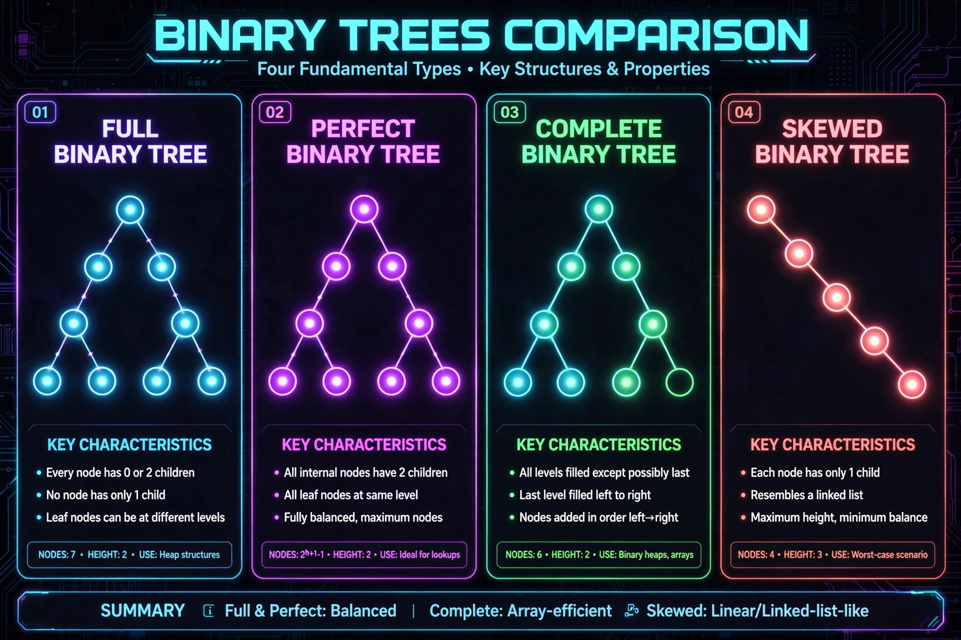
Most data structures we learn at the beginning organize information linearly: a list, an array, a queue. But the real world is not linear. Your computer's file system is hierarchical. A company's organizational chart is hierarchical. The DOM of a web page is hierarchical. To represent these structures, we need something more than a list: we need trees.

A binary tree is the most fundamental and elegant form of hierarchical structure in computing. It is a non‑linear data structure in which each node has at most two children, conventionally called the left child and right child. This constraint — "at most two" — is what makes it so powerful and, at the same time, so manageable.

But do not be fooled by its apparent simplicity: binary trees are the basis of the fastest search systems (binary search trees), database engines (B‑Trees), data compression (Huffman coding), compilers (abstract syntax trees), and even artificial intelligence (decision trees). Understanding them is not just an academic exercise; it is understanding how a fundamental part of the software you use every day works.

How does a binary tree work?

The basic structure

A binary tree is composed of nodes. Each node contains three fundamental elements:

A value (the data it stores)
A reference to the left child
A reference to the right child

The top node, from which the entire tree hangs, is called the root. Nodes with no children are called leaves. Intermediate nodes are internal.

Key terminology

Parent: the node immediately above another
Child: the node immediately below another
Siblings: nodes that share the same parent
Ancestor: any node on the path from the root to a given node
Descendant: any node on the path from a given node to a leaf

Two essential metrics: depth and height

The depth of a node is the length of the path from the root to that node (counting edges). The height of a node is the length of the longest path from that node to a leaf. The height of a tree is therefore the height of its root.

flowchart TD
    A["RootDepth: 0"] --&gt; B["Internal nodeDepth: 1"]
    A --&gt; C["Internal nodeDepth: 1"]
    B --&gt; D["LeafDepth: 2"]
    B --&gt; E["LeafDepth: 2"]
    C --&gt; F["LeafDepth: 2"]
    C --&gt; G["LeafDepth: 2"]
    
    style A fill:#e3f2fd,stroke:#1565c0
    style B fill:#e8f5e9,stroke:#2e7d32
    style C fill:#e8f5e9,stroke:#2e7d32
    style D fill:#fff3e0,stroke:#ef6c00
    style E fill:#fff3e0,stroke:#ef6c00
    style F fill:#fff3e0,stroke:#ef6c00
    style G fill:#fff3e0,stroke:#ef6c00

Traversals: the three ways to visit a binary tree

To process a binary tree, we need to traverse it. There are three classic traversals, each with a different order:

Preorder: visit the root node, then the left subtree, then the right.
Inorder: visit the left subtree, then the root, then the right.
Postorder: visit the left subtree, then the right, then the root.

flowchart LR
    subgraph Preorder["Preorder: A → B → D → E → C → F → G"]
        P1["A"] --&gt; P2["B"]
        P1 --&gt; P3["C"]
        P2 --&gt; P4["D"]
        P2 --&gt; P5["E"]
        P3 --&gt; P6["F"]
        P3 --&gt; P7["G"]
    end

    subgraph Inorder["Inorder: D → B → E → A → F → C → G"]
        I1["A"] --&gt; I2["B"]
        I1 --&gt; I3["C"]
        I2 --&gt; I4["D"]
        I2 --&gt; I5["E"]
        I3 --&gt; I6["F"]
        I3 --&gt; I7["G"]
    end

    subgraph Postorder["Postorder: D → E → B → F → G → C → A"]
        O1["A"] --&gt; O2["B"]
        O1 --&gt; O3["C"]
        O2 --&gt; O4["D"]
        O2 --&gt; O5["E"]
        O3 --&gt; O6["F"]
        O3 --&gt; O7["G"]
    end

Why is this data structure so famous?

Binary trees are famous for one fundamental reason: they allow logarithmic‑time operations when used correctly. A balanced binary tree of n nodes has a height of O(\log n). This means that searching, inserting, or deleting an element in a well‑balanced binary search tree takes, in the worst case, time proportional to \log n — much faster than a linked list (O(n)) and with a performance guarantee that hashing does not always offer.

Their real‑world applications are countless:

File systems: directories and subdirectories are trees.
Databases: B‑Tree and its variants are generalized binary trees.
Compilers: syntactic analysis generates abstract syntax trees.
Artificial intelligence: decision trees are the basis of many machine learning algorithms.
Data compression: Huffman coding uses binary trees.
Networks: routing algorithms use trees.

flowchart LR
    subgraph Applications["Applications of binary trees"]
        FS["File systems"]
        DB["Databases"]
        COMP["Compilers"]
        AI["Artificial Intelligence"]
        ZIP["Data compression"]
        NET["Networks"]
    end
    
    FS --&gt; BT["Binary Trees"]
    DB --&gt; BT
    COMP --&gt; BT
    AI --&gt; BT
    ZIP --&gt; BT
    NET --&gt; BT
    
    style BT fill:#e1f5fe,stroke:#0288d1

Types of binary trees

Not all binary trees are the same. There are variants with specific properties that make them suitable for different problems.

Full Binary Tree

Every node has 0 or 2 children. No node has only one child. All internal nodes have exactly two children and all leaves are at the same level.

flowchart TD
    A["A"] --&gt; B["B"]
    A --&gt; C["C"]
    B --&gt; D["D"]
    B --&gt; E["E"]
    C --&gt; F["F"]
    C --&gt; G["G"]

Perfect Binary Tree

It is a special case of a full tree: all internal nodes have two children and all leaves are at the same depth. Its number of nodes is 2^{h+1} - 1, where h is the height.

Complete Binary Tree

All levels, except possibly the last, are completely filled, and the nodes on the last level are as far left as possible. This is the structure used in heaps.

flowchart TD
    A["A"] --&gt; B["B"]
    A --&gt; C["C"]
    B --&gt; D["D"]
    B --&gt; E["E"]
    C --&gt; F["F"]

Binary Search Tree (BST)

It is a binary tree with an additional property: for each node, all values in its left subtree are less than the node's value, and all values in its right subtree are greater. This enables fast searches: at each step, you discard half the tree.

Balanced Binary Tree

A binary tree is balanced if, for each node, the height of its left and right subtrees differs by at most 1. The best‑known variants are AVL trees and Red‑Black trees.

Skewed Binary Tree

This is the degenerate case: each node has only one child. In practice, the tree behaves like a linked list, with O(n) complexity.

flowchart TD
    A["A"] --&gt; B["B"]
    B --&gt; C["C"]
    C --&gt; D["D"]
    D --&gt; E["E"]

Mathematics of binary trees

Like any data structure, binary trees can be described with mathematical precision. These are the fundamental formulas.

Maximum number of nodes

In a binary tree of height h (where the root is at level 0), the maximum number of nodes is:

N_{\text{max}} = 2^{h+1} - 1

This is because each level i can have at most 2^i nodes.

Minimum number of nodes

The minimum number of nodes for a height h is:

N_{\text{min}} = h + 1

This occurs in a skewed tree, where each level has exactly one node.

Relationship between nodes and height

For a binary tree with n nodes, the minimum possible height is:

h_{\text{min}} = \lceil \log_2(n+1) \rceil - 1

And the maximum possible height is:

h_{\text{max}} = n - 1

Number of leaf nodes

In a full binary tree (where every node has 0 or 2 children), the number of leaves L and the number of internal nodes I satisfy:

L = I + 1

This is a fundamental property of full binary trees.

Average depth

For a binary search tree built from random insertions, the expected depth of a node is approximately:

2 \ln n \approx 1.39 \log_2 n

This explains why random BSTs perform so well in practice, even without explicit balancing.

Binary trees in code

Let us see how to implement a binary tree in the most popular languages. All examples share the same structure: a Node class with a value and two child references.

Java

public class BinaryTree {
    static class Node {
        T value;
        Node left;
        Node right;
        
        Node(T value) {
            this.value = value;
            this.left = null;
            this.right = null;
        }
    }
    
    private Node root;
    
    public BinaryTree() {
        this.root = null;
    }
    
    // Preorder traversal
    public void preorder() {
        preorder(root);
    }
    
    private void preorder(Node node) {
        if (node == null) return;
        System.out.print(node.value + " ");
        preorder(node.left);
        preorder(node.right);
    }
}

Python

class Node:
    def __init__(self, value, left=None, right=None):
        self.value = value
        self.left = left
        self.right = right
    
    def __repr__(self):
        return f"Node({self.value})"

class BinaryTree:
    def __init__(self):
        self.root = None
    
    def preorder(self, node=None):
        if node is None:
            node = self.root
        if node is None:
            return
        print(node.value, end=" ")
        self.preorder(node.left)
        self.preorder(node.right)

JavaScript

class Node {
    constructor(value) {
        this.value = value;
        this.left = null;
        this.right = null;
    }
}

class BinaryTree {
    constructor() {
        this.root = null;
    }
    
    preorder(node = this.root) {
        if (node === null) return;
        console.log(node.value);
        this.preorder(node.left);
        this.preorder(node.right);
    }
}

C#

public class BinaryTree
{
    public class Node
    {
        public T Value { get; set; }
        public Node Left { get; set; }
        public Node Right { get; set; }
        
        public Node(T value)
        {
            Value = value;
            Left = null;
            Right = null;
        }
    }
    
    private Node _root;
    
    public BinaryTree()
    {
        _root = null;
    }
    
    public void Preorder()
    {
        Preorder(_root);
    }
    
    private void Preorder(Node node)
    {
        if (node == null) return;
        Console.Write(node.Value + " ");
        Preorder(node.Left);
        Preorder(node.Right);
    }
}

Rust

use std::rc::Rc;
use std::cell::RefCell;

#[derive(Debug)]
struct Node {
    value: T,
    left: Option&gt;&gt;&gt;,
    right: Option&gt;&gt;&gt;,
}

impl Node {
    fn new(value: T) -&gt; Rc&gt; {
        Rc::new(RefCell::new(Node {
            value,
            left: None,
            right: None,
        }))
    }
}

struct BinaryTree {
    root: Option&gt;&gt;&gt;,
}

impl BinaryTree {
    fn new() -&gt; Self {
        BinaryTree { root: None }
    }
}

The poll: which data structure would you choose?

Imagine you are building a system that must handle hierarchical data with frequent search, insertion, and deletion operations, and you need performance to be predictable and efficient even in the worst case. Which data structure would you choose?

Which data structure would you use for this problem?

References

Real Python. (2026, June 22). binary tree | Computer Science Glossary. https://realpython.com/ref/computer-science-glossary/binary-tree/
Zeil, S. J. (2026, March 16). 1 Tree Terminology. Old Dominion University. https://cs.odu.edu/~zeil/cs361/live/Public/treedefinitions/treedefinitions__slides.html
Zeil, S. J. (2026, March 2). Balanced Search Trees. Old Dominion University. https://www.cs.odu.edu/~zeil/cs361/s26-webss/Public/avl/index.html
Educative. (2026). Introduction to Trees Including Binary and Balanced Trees. https://www.educative.io/courses/data-structures-coding-interviews-python/np/overview-of-trees
CS61B Textbook. (2026, Spring). 15.2 BST Definitions. https://cs61b-2.gitbook.io
Glavic, B. (2021). Binary Search Trees. Illinois Institute of Technology. http://www.cs.iit.edu/~glavic/cs331/2021-spring/notebooks/binary-search-trees.ipynb